What is the most complex AI model that we fully understand?

While many people have a feeling that AI technology is 'somehow incomprehensible,' even those who are familiar with it seem to share the same sentiment.
The most complex model we actually understand - YouTube
The tokens generated by the AI are the result of tens of billions of calculations, and the parameters used in the calculations have been learned by training the AI to predict one token at a time.
However, no one has a definitive answer to the question of how something resembling true intelligence can emerge from repeatedly learning to predict small pieces of text over and over again through trillions of examples. The mechanisms of the individual
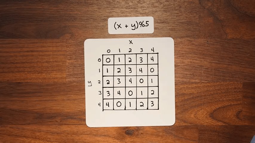
In 2021, OpenAI researchers trained a small model to perform modular arithmetic, which allows mathematical operations like 'x + y' to be transformed into datasets.
・Prepare a grid with x columns and y rows
- Place various x values in the columns and various y values in the rows
・Set the sum of the x and y values in the cell where the row and column intersect
- There is a maximum value for the cell value, and if the value you try to set exceeds the maximum value, the remainder when divided by the maximum value is set.
The AI model is interested in learning about this modulo operation, so it reserves only a portion of the data for testing and uses the rest for training. From the AI model's perspective, five tokens are needed to represent the numbers 0 through 4, plus one token to represent the equal sign. The plus token is unnecessary because this training only involves addition. For example, when inputting the arithmetic problem '1 + 2' into the model, the first token '1' in the problem is passed to the model by turning on only the 1 position and turning off all other positions. The second token '2' turns on only the second input. The final equal sign turns on only the sixth input. Therefore, from the model's perspective, the arithmetic problem '1 + 2' is input in the following order: only the first token is turned on, then only the second token is turned on, then only the sixth token is turned on. Furthermore, because the Transformer model is configured to return an output with the same dimensions as the input, the final output of the model is also 6x3.
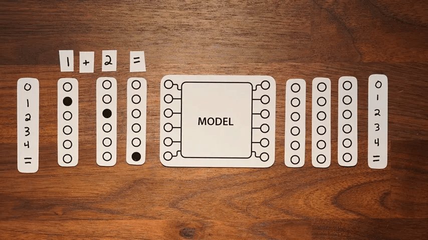
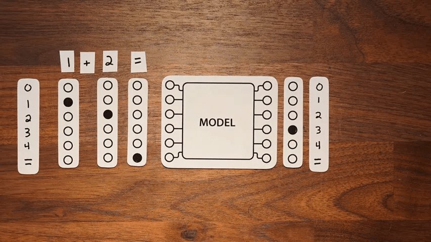
However, in this model, only the last column output is needed. In the '1 + 2 = 3' example, the third output in the last column will be turned on.
In other words, what the model is learning is mapping a pattern of 18 values to a new pattern of 6 values.

Similarly, various target input and output patterns are given, such as '1 + 3 = 4' or '2 + 3 = 0.' By observing these examples thoroughly, the underlying structure of the problem can be understood, which is the precise operating principle of large-scale language models.

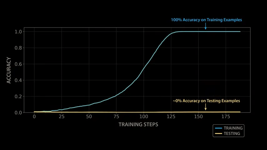
When the OpenAI team trained a model with modular arithmetic, the initial results were quite disappointing: although the model was able to quickly learn the patterns in the training data and produce correct outputs for all training examples, it performed extremely poorly on the test set - it appeared that the model had not actually learned modular arithmetic, but had simply memorized the training data by rote.
However, one researcher made the mistake of leaving a trained model on vacation, and after numerous training steps during the vacation, the model
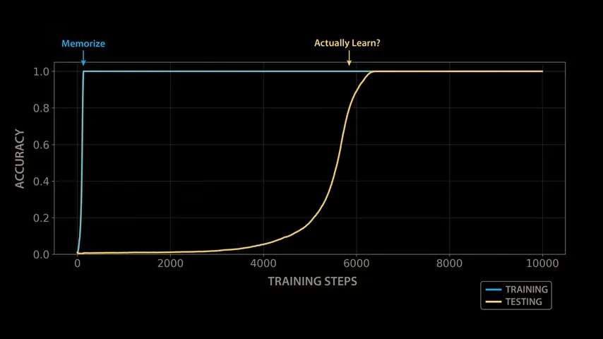
The OpenAI team succeeded in reproducing the sudden generalization phenomenon in various arithmetic operations and model configurations, and published a paper on this phenomenon titled '
Grokking: Generalization Beyond Overfitting on Small Algorithmic Datasets
https://arxiv.org/abs/2201.02177

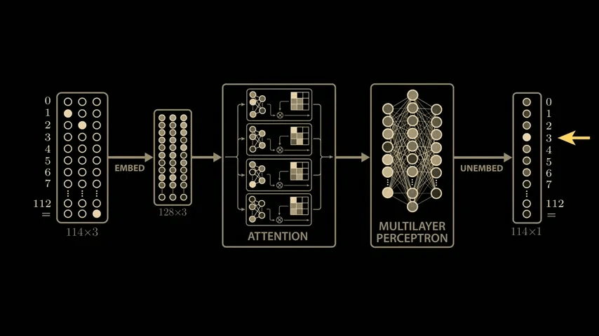
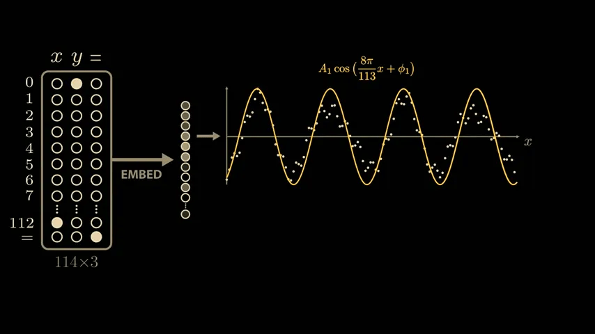
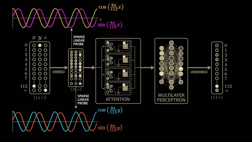
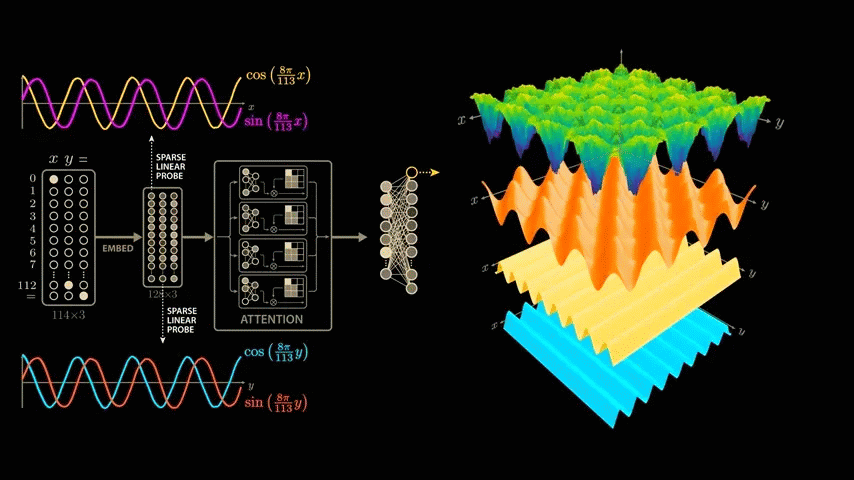
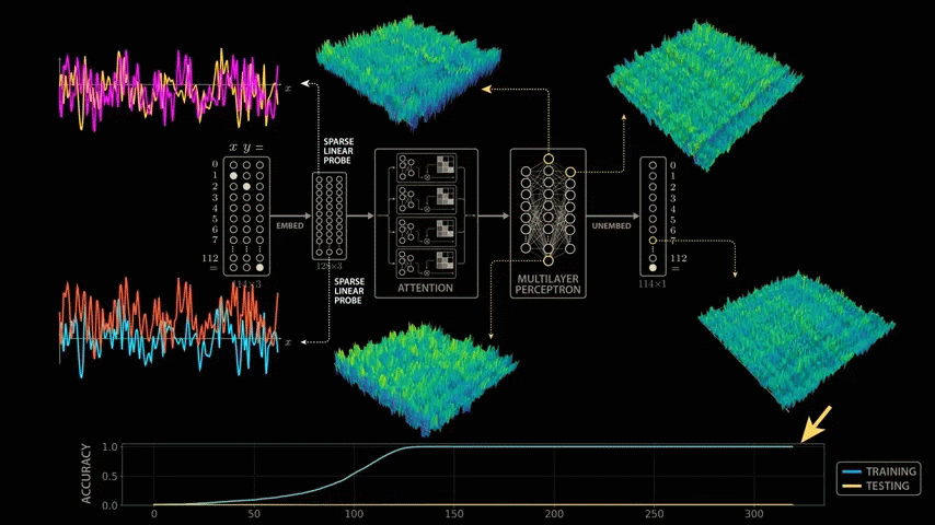
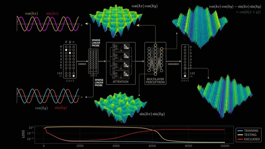
The paper delves deeply into the model's parameters and activations, and derives a highly convincing and elegant explanation. While the paper's model is larger than the simplified model mentioned above, it uses 113 digits in NAND. Therefore, the model's input vector is 114 in length, consisting of 113 points representing the numbers 0 to 112 and one point representing the equal sign. To calculate '1 + 2,' the model is passed this 114x3 matrix. The matrix contains a 1 in the first position of the first column, a 1 in the second position of the second column, a 1 in the equal sign position of the last column, and all other positions are 0. The input 113x3 matrix is then multiplied by the trained weight matrix (embedding matrix) to generate a new 128x3 vector. The embedding vector is passed through
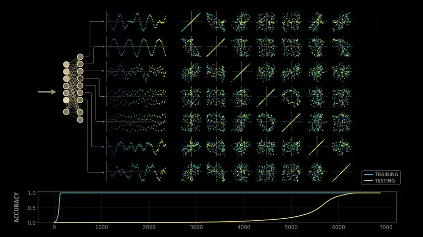
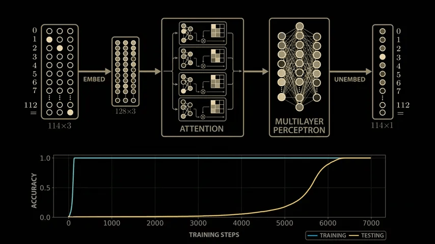
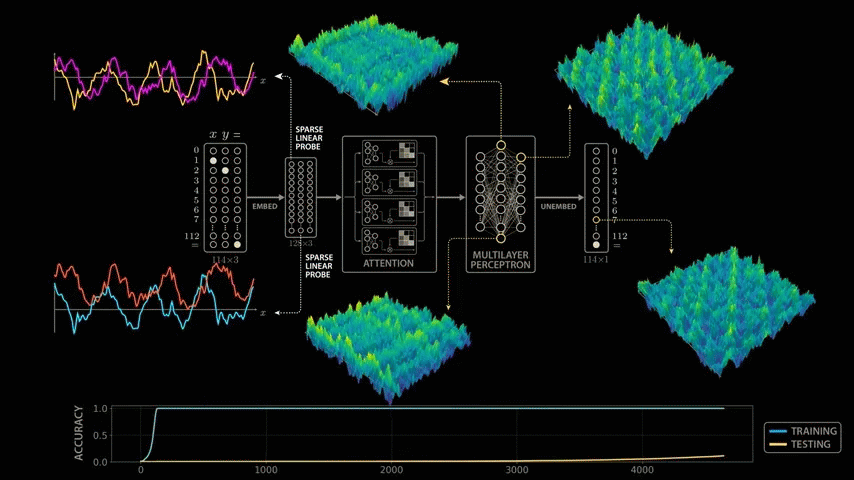
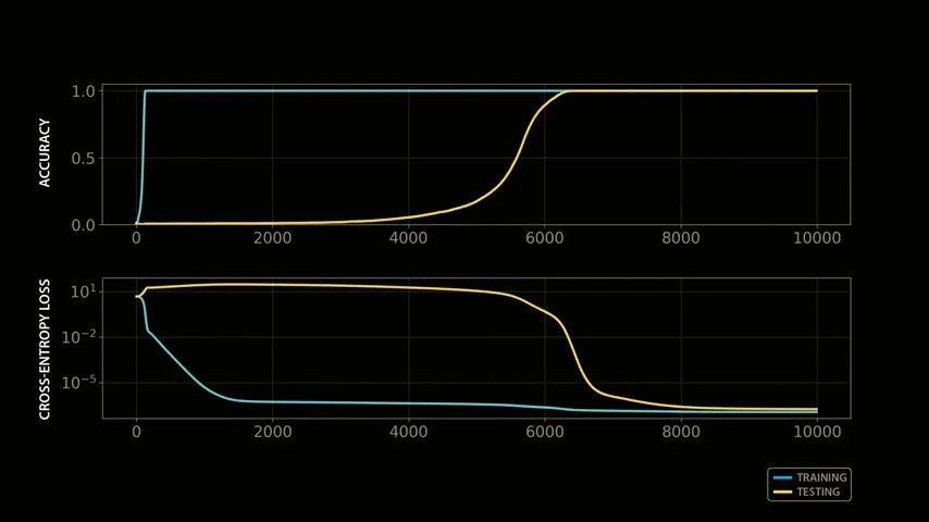
Training the model with modular arithmetic shows the same growth pattern observed by the OpenAI team: the model memorizes the training data after about 140 steps and generalizes after 10,000 training steps.
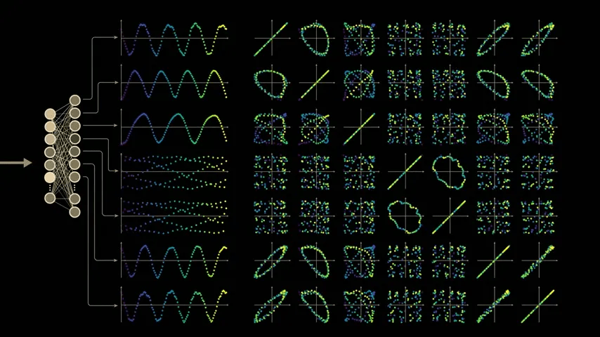
To take a closer look at the intermediate outputs (activations) of the model, we take a closer look at the outputs of the 512 neurons in the second layer of the multi-layer perceptron block.
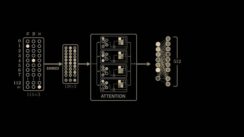
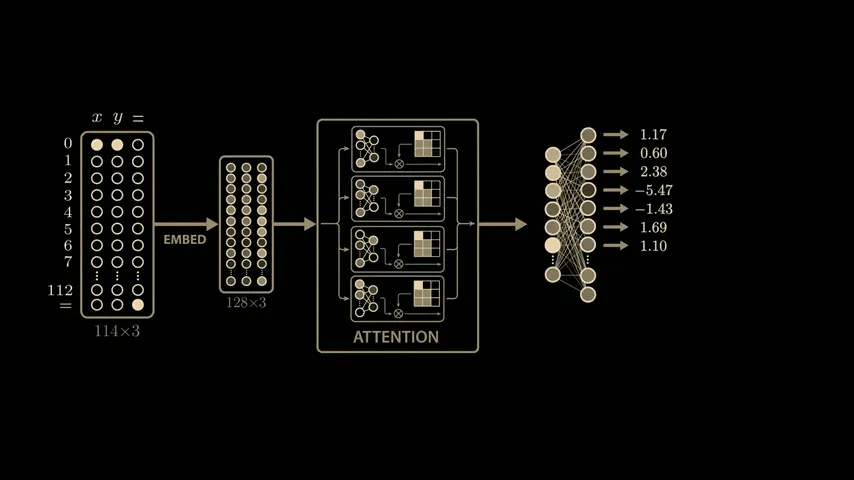
If you feed the network the problem '0 + 0,' the first neuron in this layer will return an output value of 1.17, the second neuron will return 0.6, and so on.
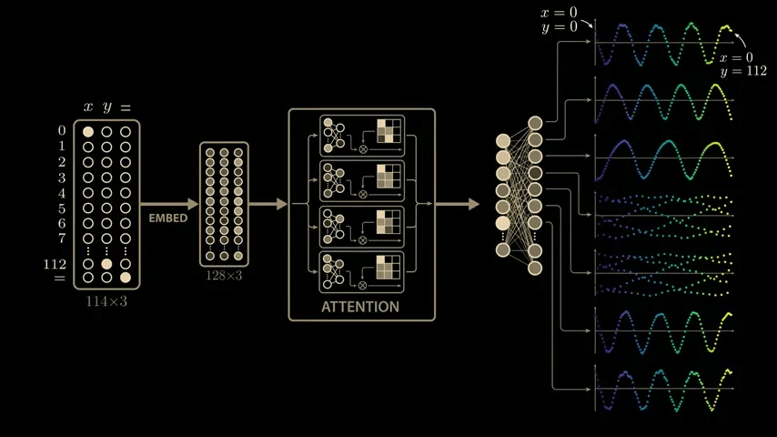
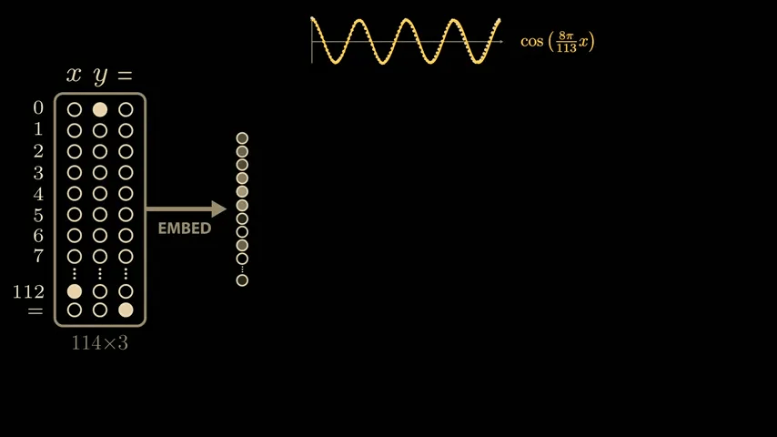
Now let's visualize the change in values when the input formula is changed. Fix the value of x to 0 and explore the range of y values. Proceeding with '0 + 0,' '0 + 1,' '0 + 2,' and so on, we cover all 113 possible values of y, and a sine wave-like shape will appear in some of the neuron outputs.
To investigate further, we can explore the correlations between all pairs of these neurons by creating a scatter plot of each pair of neurons in a 7x7 grid. For example, in the second scatter plot (first row), we plot the output of the first neuron as the y value and the output of the second neuron as the x value. The plot forms a beautiful loop.
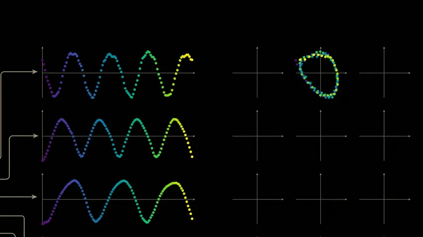
As we make similar plots for each neuron output pair, we can see that the model clearly exhibits some structure.
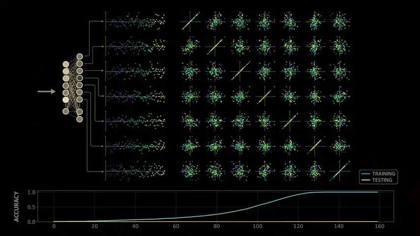
However, I am curious as to whether this structure is related to learning, so I will look back at the training and check.
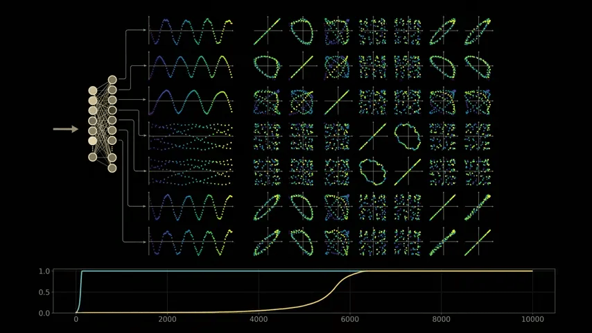
We can see that these structures completely disappear at the model stage where the training data is simply memorized. In other words, the initial model does not show any waveforms or loops that appear after training, so this may be related to the training stage.
The waveforms and loops the model generates internally during the groping behavior suggest that it may be calculating and utilizing the sine and negativity of the inputs x and y. Applying
Plotting these waves on the model output shows excellent agreement.
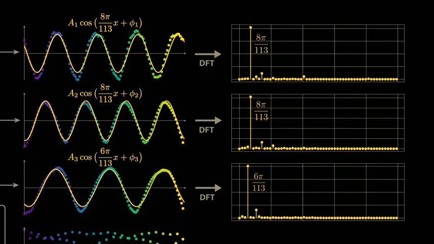
To identify whether the waveforms shown by the model are due to training, we use a technique called ' sparse linear probing .' By sampling a few more values in the embedding vector, we can see similar semi-periodic curves.
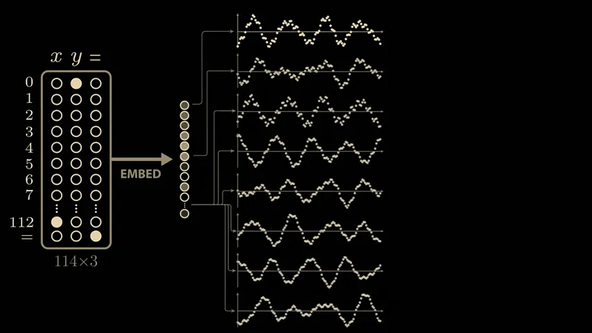
It turns out that connecting the eight curves with
At this stage, we can calculate a similar sparse linear probe for the sin value of x × 8π/113.
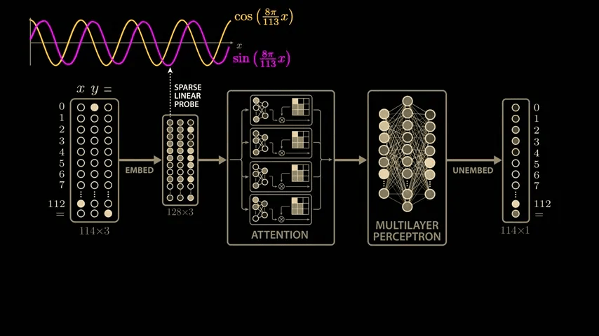
The first embedding vector depends only on the first input, x, and the second embedding vector depends only on the second input, y. These inputs are combined in the attention block, but because the same embedding matrix is used to process the three inputs independently, we can apply the same sparse linear probe to the second embedding vector. When we do, we see the same beautiful cosine and sine curves, but this time as a function of y. This means that the model learns to compute the sine and cosine of its inputs very early on.
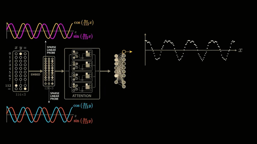
Now let's explore how these outputs change when we vary both x and y, to see if we can figure out how the network connects these variables. If we graph the output of a single neuron, fix y to 0, and scan all possible values of x, we get the familiar cosine curve.
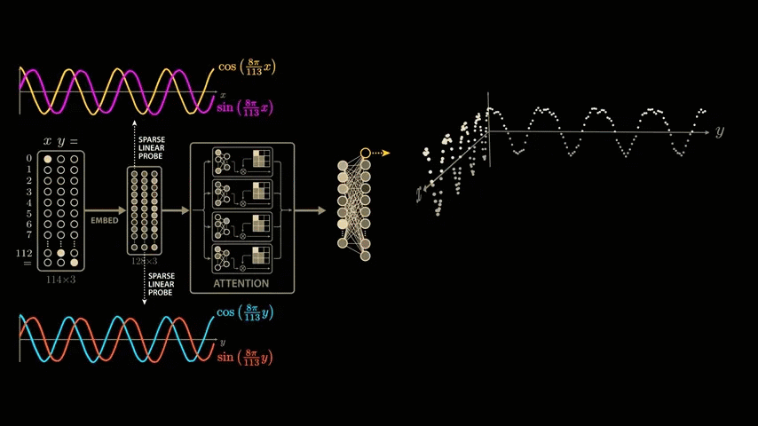
Next, we add an axis to the graph and plot the neuron's output while varying y.
We explore all combinations of x and y and plot the neuron's output as the height of
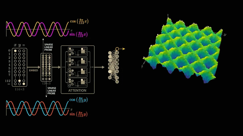
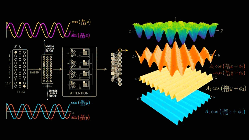
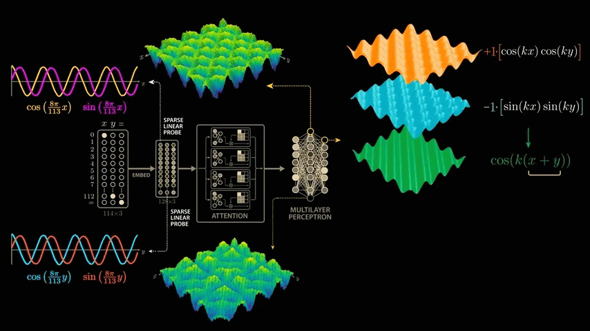
To find the combination of sine and cosine curves that best captures this wave structure that the network has learned, we again apply the Discrete Fourier Transform, but this time to both x and y.
By extracting the higher frequencies, we can decompose the surface graph into several major components. In the decomposition graphs below, the component in the bottom blue graph is cos(x), the component in the second graph from the bottom yellow graph is cos(y), and the component in the third graph from the bottom orange graph is the strongest and most interesting because it is equal to the product of cos(x) and cos(y).
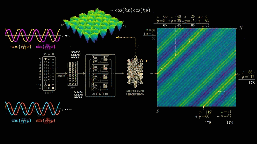
Now let's go one layer deeper into the multilayer perceptron and plot the output of the neurons in this layer as a function of x and y. We can see the same wave-like shape, but the waves are more irregular and diagonal than before.
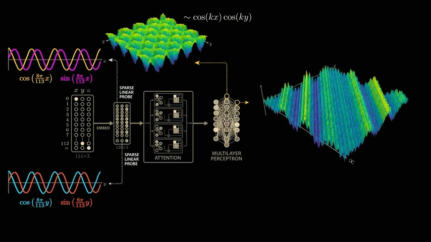
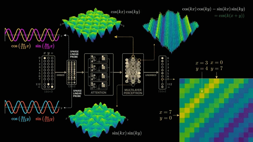
For the two wave crests where the neuron's output is maximized, we look at the combination of input values that corresponds to the wave crest.
The first crest of the first wave is x = 0, y = 65. Moving down and to the left along the crest, the intermediate values are x = 20, y = 45, x = 40, y = 25, x = 60, y = 5, and finally x = 65, y = 0. All input pairs sum to 65. This means that the neuron fires maximally when x + y equals 65. Thus, the neuron has uniquely learned to add, or more precisely, it fires for all input pairs that sum to 65.

The second wave peak begins at 'x = 66, y = 112', passes through values such as 'x = 91, y = 87', and ends at 'x = 112, y = 66', all of which add up to 178. Considering that the model was trained on modulo arithmetic with a divisor of 113, the second wave peak also consists of an input pair that adds up to 65.
So how does a single layer of neurons go from cos(x) × cos(y) to adding x and y themselves?
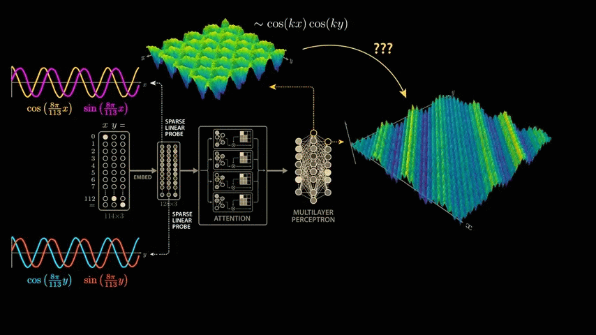
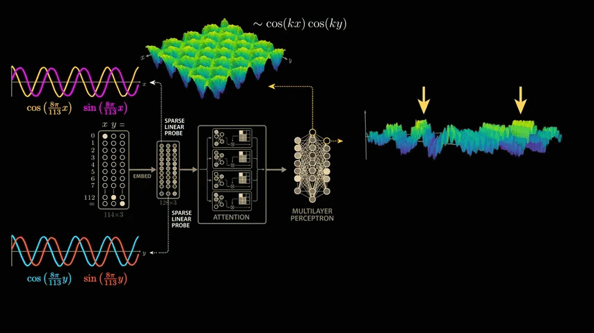
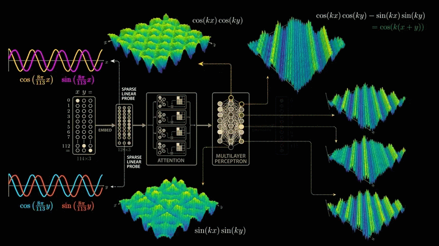
We have just confirmed that the strongest frequency component in the output of layer 1 neurons is cos(x) × cos(y), and the strongest frequency component in the output of layer 2 neurons is sin(x) × sin(y). Now we make the following assumptions:
The weight assigned to the cos(x) × cos(y) neuron is 1 .
The weight assigned to the sin(x) × sin(y) neuron is -1 .
The negative weights flip the second graph upside down, and now when we add the weighted graphs together, the sin and cos interact in a surprising way to create the diagonal symmetry we see in the next layer of neurons, which fire on combinations of inputs that sum to 65.
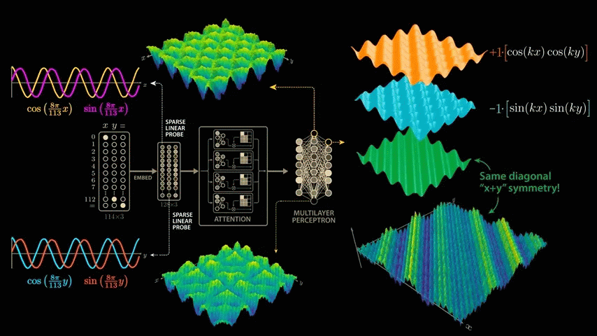
cos(x) × cos(y) - sin(x) × sin(y) is actually the trigonometric formula '
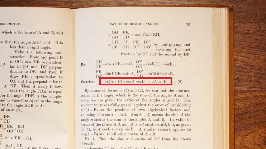
Amazingly, the network appears to have learned to effectively exploit this trigonometric formula to solve modular arithmetic.
The final unbounded part of the model further computes a weighted sum. This time, we look at the output of the final layer neurons in a multilayer perceptron. Graphing the output of several neurons reveals diagonal symmetry with various shifts and scales.
Below is the resulting surface graph where the output returns 7.
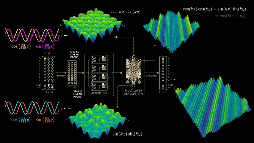
Similar to the multilayer perceptron neuron that found all combinations of numbers that add up to 65, this graph reaches a maximum for all combinations of x and y that add up to 7. To solve this modular multiplication problem, the network estimates the signs and proximity of the input numbers and calculates the product of these functions. It then cleverly uses trigonometric formulas to create the diagonal symmetry needed to solve the modular multiplication problem, and combines multiple of these resulting patterns to arrive at the final answer.
To understand why the model grows by taking a closer look at how it solves modular arithmetic, let's revisit the training process, visualizing the evolution of the various structures the model learns. After a few hundred steps, the model perfectly fits the training data, but still shows no signs of generalization or affinity.
As training progresses, the model's performance plateaus, making it seem like nothing is happening. It's common to visualize training and test performance during model training, and if both metrics remain stable for such a long period of time, one would normally assume that training is complete and the model has converged to a stable solution. However, a closer look under the hood reveals that the model is beginning to assemble the necessary structures to solve the modular arithmetic problem.
In their paper,
Now that we know the model is operating at a few dominant frequencies, we can remove information about those dominant frequencies from the model's final output before measuring performance. That is, we remove the 8π/113 frequency we discovered earlier, and plot this removal loss over the training process. The new metric drops sharply with training loss, but then gradually rises as the model builds up sine and cosine curves. The reason the removal loss increases is because we've removed the model's ability to utilize those dominant frequencies.
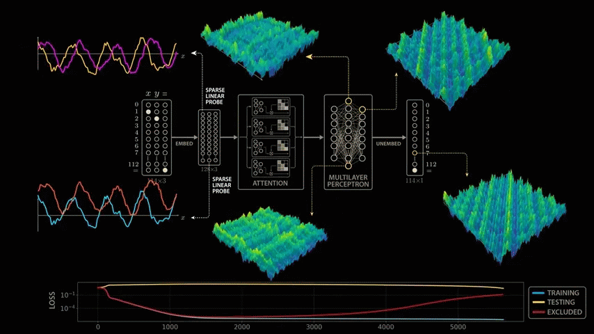
Notably, the elimination loss gradually increases over time, even as training and testing performance plateaus, indicating that the model increasingly exploits dominant frequency patterns. Interestingly, Nanda et al. suggest that growth does not occur upon completion of the sin-cos structure, but rather immediately after the 'cleanup phase,' in which the model removes memory examples that were reliant on during initial training. This dynamic is extremely intriguing and clearly explains why the model achieves superior performance in modular arithmetic. The elimination loss metric clearly demonstrates the model's gradual progression from memory reliance to learning, and elegantly explains the glocking phenomenon. This clarity is a beautiful yet rare anomaly in modern AI, a rare 'transparent box' in a world of black boxes.
Related Posts: